3. Assessment Procudure
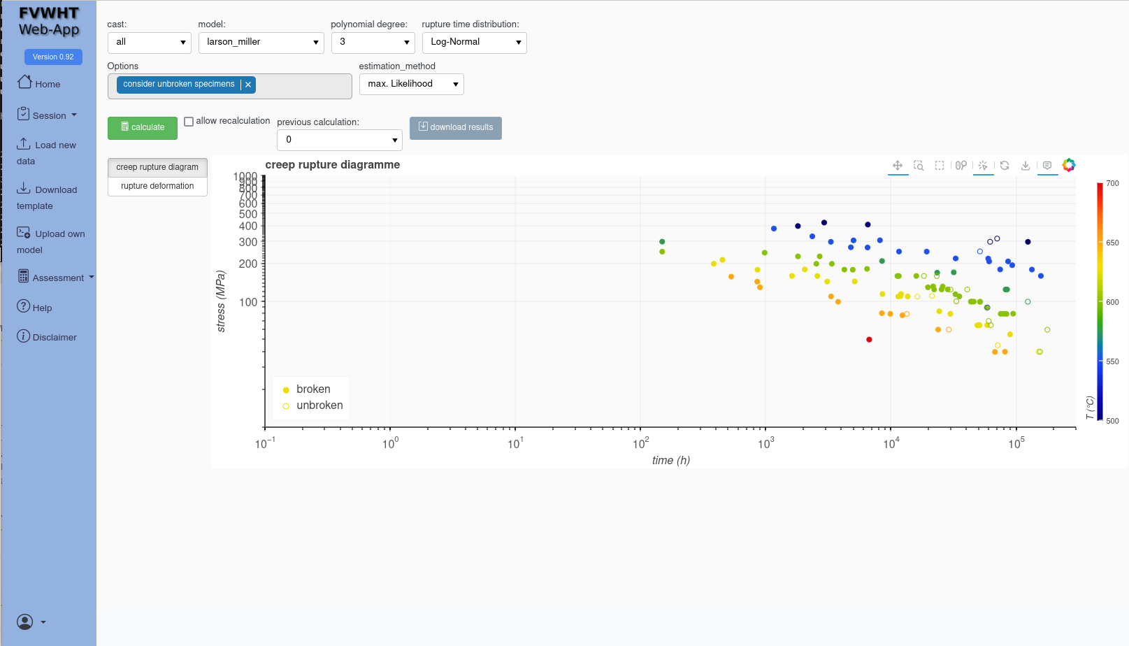
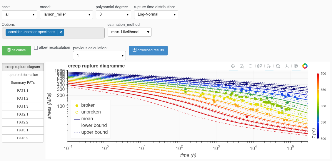
The test durations of the failed and unfailed creep rupture tests from the input file are plotted in a creep strength diagramme.
3.1. Prepare the calculations
With the pull-down menu “model” you can selct the model type for the creep rupture data assessment (CRDA)
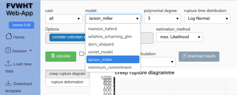
The following model types are implemented:
Based on time temperature parameters:
Larson-Miller
Manson-Haferd
Dorn-Shepard
For the time temperature parameters you can choose the polynomial degree of the polynomal:
with
Algebraic functions
Soviet Model
Minimum Committment
Wilshire-Scharning
You can also select the distribution functions:
Log Nomal distribution
Weibull distribution (two-parameter)
Log-Logistic distribution
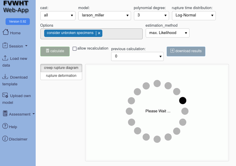
3.2. Perform the calculations
After you selected the the model type and distribution functions, you can start the assessment with the button “calculation”. Depending on the parameters selected and the number of data points in the input file, the calculation takes approx. 3 to 10 seconds. The calculations are carried out for the full data set of the input file and for the thinned data sets for PAT3.1 and PAT3.2. A total of 3 complete model adjustments are therefore always carried out. Depending on the parameters selected and the number of data points in the input file, the calculation takes approx. 3 to 10 seconds. The calculations are carried out for the full data set of the input file and for the thinned data sets for PAT3.1 and PAT3.2. A total of 3 complete model adjustments are therefore always carried out. During the calculations, the website indicates that the result is being awaited.
After finishing the calculations , the result is shown in the plot.
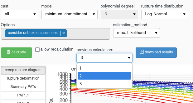
You can repeat the calculation with other parameters or other model functions. Each new calculation with the loaded input data set is saved in the session and placed on a stack that can be called up via the “previous calculation” pull-down menu.